The experience curve: how BCG turned falling costs into a strategy

In 1963 Black & Decker sold its quarter-inch drill for $15.98. By 1970 the price was $7.99. Over roughly the same years, company sales went from over $100 million in 1964 to past $200 million in 1969 and more than $500 million in 1974, according to Walter Kiechel’s history of the strategy business, The Lords of Strategy.

Francis Lucier, the executive who ran that push, described the pricing logic to Kiechel in one line: “What we were doing was pricing it for what it was going to be.” Kiechel recounts that Lucier got the idea from Bruce Henderson of the Boston Consulting Group, after attending BCG’s conferences and inviting Henderson to present to Black & Decker’s executives. The idea was that the more of something you make, the cheaper each unit gets, at a rate predictable enough to plan around. BCG called it the experience curve, and Kiechel calls it “the single most important concept in launching the strategy revolution.”

BCG took an aircraft-factory rule and applied it to every cost a company has

The starting point was the learning curve, and Kiechel describes the evidence BCG found in a 1964 Harvard Business Review article by Winfred Hirschmann:

As Hirschmann noted, as early as 1925, manufacturers of aircraft had begun to observe that the amount of labor that went into making an aircraft declined predictably as the number of planes manufactured increased. Typically, the fourth plane took only 80 percent of the labor required to make the second, the eighth only 80 percent of what had gone into the fourth.

In Kiechel’s account, BCG devised the curve in 1966. A client, General Instruments, was struggling to match competitors’ prices on television components, and Henderson sent a young consultant, John Clarkeson, to find out why and to gather whatever literature he could find on the learning curve. Henderson’s own history of the idea, “The Experience Curve—Reviewed, II. History,” written for BCG’s Perspectives series in 1973, says the clinching evidence came from semiconductor prices compared with accumulated industry volume. BCG found that “prices, in constant dollars, declined steadily at a constant rate of about 25 percent each time accumulated experience doubled. That was the experience curve. That was 1966.”

The older learning curve, Henderson notes in the same essay, “only applied to direct labor.” His 1968 Perspectives essay, “The Experience Curve”, widened it to everything needed to get the product to the customer: “There is no question that R & D, sales expense, advertising, overhead, and everything else is included.” BCG also tied the curve to competition, a step Kiechel calls “vastly more important”:

BCG posited a direct relationship between a company’s position on the experience curve—and hence its costs—and its market share. The competitor with the largest share, the one that sold more of the product than anyone else did, should be the one with the most “experience.”

The experience curve makes three claims:

1. Unit cost falls by a fairly steady percentage every time cumulative volume doubles. Henderson put the decline at “consistently 20-30%” per doubling in 1968. Kiechel puts BCG’s figure at “typically between 15 and 25 percent.”
2. Prices follow costs down when there’s competition. Kiechel’s summary of the early Perspectives essays: “If there’s any competition in a market, prices will eventually go down as fast as costs.”
3. The competitor with the most cumulative volume should have the lowest costs, which makes market share a cost position. Porter points out in Competitive Strategy that BCG’s growth-share matrix rests on this, on “the underlying assumption that the experience curve … is operating and that the firm with the largest relative share will thereby be the lowest cost producer.”

Henderson didn’t think the decline happened by itself. The same 1968 essay says the cost reductions “are not necessarily automatic. They depend crucially on a competent management that seeks ways to force costs down as volume expands.”

Each doubling cuts cost by the same share, so later savings take far more volume

The curve is about cumulative volume, every unit the company has ever made, not volume per year. On an 80 percent curve, unit 2 costs 80 percent of unit 1, unit 4 costs 64 percent, and unit 8 costs about 51 percent. Cost halves roughly every eightfold increase in total output.

Going from 1,000 units to 2,000 takes another 1,000. Going from 10 million to 20 million takes another 10 million. Henderson spelled out what that means for a business that stops growing: “If the production of a product is not growing, then the rate of cost decline per year gradually slows down and approaches zero.”

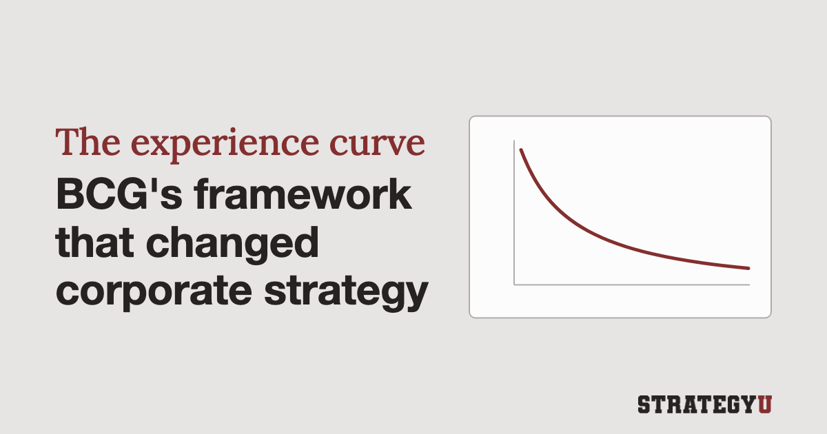
Plotted on ordinary axes, the curve drops steeply and then flattens. On log scales, where each doubling covers the same distance, it becomes a straight line, and the steeper the line, the faster costs fall per doubling. Use the mock case below to see how the rate changes the shape, then switch to fifty years of real solar data.

The real data uses Our World in Data’s series, which shows solar module prices falling from about $132 per watt in 1975 to about $0.27 in 2024 (in constant 2025 dollars). Over the same years, cumulative installed capacity grew from about half a megawatt to more than 1.8 million megawatts, roughly 22 doublings. A straight-line fit on log scales gives a decline of about 24 percent per doubling, within the range Henderson described in 1968.¹ The fit for 2004 to 2024 alone is steeper, around 30 percent.

IRENA’s Renewable Power Generation Costs in 2025 reports that “Module prices sold in Europe reached their lowest levels ever in 2025” and that “By the end of 2025, module prices had reached a floor with little room for further cost reduction.” In 2026 they rose. pvXchange’s index of mainstream modules sold in Europe went from €0.105 per watt in January to €0.130 in September, up 23.8%. The chart’s open circles estimate 2025 and 2026, and both still sit below the 50-year trend line, where module prices have been every year since 2013.²

Pricing ahead of the curve was BCG’s central prescription

Henderson’s 1968 essay drew the pricing implication directly: “New products should be priced as low as necessary to dominate their market segment or probably not be sold at all.” Porter names Texas Instruments, Black & Decker, and Emerson Electric as firms that built successful strategies on the curve, “often by pricing in anticipation of future cost declines.”

Black & Decker priced its tools for the costs it expected to have

Kiechel reports that Black & Decker had found, before it met BCG, that lower prices sold far more tools. When its circular saw retailed at $30.00 to $35.00 it sold around 50,000 a year, and at $19.95 it was selling 600,000. In Kiechel’s account, the experience curve gave Lucier’s team the logic behind what they were doing and “the confidence to apply the same logic to one new product after another.”

Lucier passed on to Kiechel what friends at Stanley Tools told him about their CEO’s reaction when Black & Decker launched its Workmate workbench:

“Their CEO saw our television ads for it and yelled, ‘Jeez, that’s our business, our business. What are they doing in our business?’ But every time they’d cost the thing, they’d come back and say, ‘They’re not making any money on this.’ What we were doing was pricing it for what it was going to be. And you know what, Stanley never got into the business; it proved the point.”

Texas Instruments priced chips and calculators for costs it hadn’t reached yet

TI cut chip prices before costs or customers required it

Morris Chang, who ran TI’s integrated circuits business before founding TSMC, said in a 2007 oral history for the Computer History Museum that TI developed its semiconductor pricing “together with the Boston Consulting Group” in the late 1960s:

“The result was so called learning curve pricing. And we would automatically reduce the price every quarter. Even when the market did not demand lower price. And this was a very successful effort even though it was somewhat controversial, a lot of people think that, a lot of people thought that we were being foolish. Why do you reduce price when you didn’t have to?”

Porter, writing in Competitive Strategy in 1980, describes TI winning a market for computer memory chips before any major investments were made:

Texas Instruments announced a price for random access memories to be available two years hence. One week later, Bowmar announced a lower price. Three weeks later, Motorola announced an even lower price. Finally, two weeks after this, Texas Instruments announced a price of half of Motorola’s, and the other firms decided not to produce the product. Thus, before any major investments were actually made, Texas Instruments had won the battle.

In a footnote he adds that, for this to work, TI “must have also credibly demonstrated its commitment, from other actions, that it would actually sell memories at the low prices.”

BCG’s fifty-step cost model pointed TI to a $10 calculator

Kiechel writes that “Texas Instruments took a wilder ride down the experience curve with its personal calculator business.” In his account, J. Fred Bucy, then an ambitious TI executive, brought in BCG to study the business emerging around integrated circuits and TI’s “opportunities with calculators.” The team, led by Bill Bain with George Bennett as case manager, built experience curves for each of the fifty major activities in semiconductor production. The insight was about shared parts. A component used “in calculators, say, and in missile systems” had to be costed with experience-curve effects “calculated across all your product lines.” Bennett told Kiechel the models showed that “if you would bring out a ten-dollar calculator, and sell two or three million a year, then the reduced costs [of semiconductors] for missiles would be profound.”

The analysis, Kiechel writes, gave TI’s management “the assurance to invest in new semiconductor fabrication facilities well before TI had the actual demand in hand for the output of the ‘fabs.’”

Calculator prices fell from $150 to under $10 in four years³

Bowmar matched TI’s prices and went bankrupt

In Kiechel’s account, Bowmar was “more an assembler than an integrated manufacturer.” Electronics described it as “one of the first to market a portable electronic calculator using a single semiconductor chip (made by Texas Instruments).” Kiechel writes that when growth slowed in 1974, Bowmar matched TI’s prices. Electronics reported in February 1975 that Bowmar had filed for Chapter XI, expecting an after-tax loss of about $20 million on about $80 million of 1974 sales, and that its founder, Edward White, “blamed the losses on intense price competition as well as unusually large inventory writedowns and receivables adjustments.” The same report cited a study putting Bowmar at 12% of U.S. calculator units against TI’s 33%.

Arnoldo Hax and Nicolas Majluf used the case in a 1982 Interfaces article on experience-curve strategy. Once an industry’s early phase ends, they wrote, “the entry of new competitors generates a turbulent shakeout in the industry with a rate of price reductions much faster than the cost decline. Quite often, a complete restructuring of the industry takes place at this stage, and even the original innovator may be forced out of business. That happened to Bowmar in electronic hand calculators.”

TI survived, though Electronics reported that its second-quarter sales in 1975 fell 18% from a year earlier, and that “Declining prices and inventory adjustments in calculator operations were cited for the downturn.” Porter’s general warning in Competitive Strategy applies: “If more than one strong company is building its strategy on the experience curve, the consequences for one or more of them can be nearly fatal.”

Porter contrasts Hewlett-Packard, which he says “has erected substantial barriers based on technological progressiveness in industries in which other firms are following strategies based on experience and scale, like calculators and minicomputers.”

TI used the same pricing in watches and home computers

At the Consumer Electronics Show in Chicago in January 1976, Electronics reported, TI introduced a five-function digital watch “that will sell for $19.95—a price retailers didn’t expect until 1978.” A marketing manager at National Semiconductor called it “the most expensive advertising ploy we’ve ever seen.”

Joseph Nocera’s 1984 Texas Monthly account of TI’s home computer, the TI-99/4A, puts the strategy in one line: “Getting the volume up and the price down has always been the linchpin of TI’s sales strategy.” Nocera reports that “In just two quarters of 1983 the 99/4A cost Texas Instruments an astonishing $400 million in corporate losses.” In July 1983 it forced TI “to post the first quarterly loss in its fabled fifty-year history.” Chang, who ran TI’s consumer group for two and a half years, said in his oral history that TI started to lose its focus when it branched out into the consumer and computer businesses.

Before relying on the curve, separate experience from scale and check who can copy it

Competitors’ prices are the easiest data to plot

Kiechel writes that BCG, which couldn’t always get competitors’ cost data, “took prices as a proxy for costs” and found prices falling with cumulative volume in the pattern the learning curve predicted. Henderson’s 1973 essay describes a second pattern in the semiconductor data, prices that held steady in current dollars for long periods and then fell steeply, so a flat stretch on your chart is worth explaining before you trust the slope.

Scale advantages can be copied by building a bigger plant

Porter draws the difference: “Economies of scale are dependent on volume per period, and not on cumulative volume, and are very different analytically from experience, although the two often occur together and can be hard to separate.” Kiechel recounts, from Clayton Christensen’s research, that BCG found exactly this on a petrochemical project in the late 1960s, where the main driver of lower costs was bigger plants, so a competitor could in effect “buy” the leader’s experience by building one.

Competitors can buy experience through equipment, hires, and consultants

In Competitive Strategy, Porter lists three ways competitors can get the same experience: they copy it, hire your people, or buy “the latest machinery from equipment suppliers or purchasing know-how from consultants or other firms.” Where experience can’t be kept private, Porter writes, “new entrants may actually have an advantage,” because they can buy the newest equipment without the habits of the old way of operating.

Costs fall only when someone pushes them down

Kiechel credits Bain & Company, which Bill Bain started after leaving BCG in 1973, with turning cost reduction along the curve into a consulting practice. Steve Schaubert, a long-time Bain partner, told him: “We recognized that your costs don’t automatically decline with the experience curve. You have to manage them down.”

In a cost review, plot your unit costs against cumulative volume, compare the slope with the 20 to 30 percent Henderson described, and ask what explains the gap.

The curve fails when rivals copy the strategy, when volume grows slowly, or when technology jumps

Kiechel writes that by the early 1980s “academics and journalists were happy to proclaim the curve’s many limitations.” The abstract of George Day and David Montgomery’s 1983 Journal of Marketing article, “Diagnosing the Experience Curve”, begins: “Few strategy concepts are more likely to give misleading insights than the experience curve.” Henderson’s 1973 history had already admitted that “Understanding of the underlying causes of the experience curve is still imperfect.”

Kiechel’s own conclusion is that “none of these criticisms dispute the curve’s existence or call into question its power to discipline a company’s thinking around the imperative to cut costs incessantly.” What critics attacked, in his account, was how far the curve could be pushed. They argued “that market share didn’t necessarily equate with competitive success, that costs didn’t decline as predictably or automatically as the experience curve would have you believe, and that in some industries, a host of niche competitors thrived.”

Building ahead of the curve can wreck an industry’s returns

The summary of Pankaj Ghemawat’s 1985 Harvard Business Review article, “Building Strategy on the Experience Curve”, describes DuPont’s 1972 decision to invest $410 million over seven years to preempt competitors in titanium dioxide. By 1979, “capacity use in the industry had plummeted from 88% to 64% and Du Pont’s return on sales dropped to half its initial level of 7.5%.”

Kiechel reports that more than one early BCG consultant tells a version of the same story: a CEO whose company had cut prices to gain share and ended up in an endless price war, telling them, “You guys ruined my company.”

In slow-growing or scale-driven industries, share doesn’t buy lower costs

Kiechel’s summary of Ghemawat is that learning rates varied widely from industry to industry and that the curve was a poor guide in mature businesses like beer and cement, where cumulative volume doubles slowly. Christensen’s research, as Kiechel recounts it, also showed that in paper and textiles the consultants saw no link between market share and lower costs, because one efficient machine was enough for a competitor to match the giants.

A new technology starts a new curve

Ford built more than 15 million Model Ts between 1908 and 1927, and The Henry Ford museum notes that “the price dropped from $850 to as little as $260.”

Kiechel warns that getting locked into an experience-curve strategy can leave a company open to “being blind-sided by changes in taste or technology,” and calls the Model T everyone’s favorite example. He writes that Ford, “by pursuing an experience-curve strategy avant la lettre, … had missed the growing consumer demand for a greater variety and for close-bodied, more aerodynamic automobiles,” and lost market leadership to General Motors. Porter cites William Abernathy and Kenneth Wayne’s “Limits of the Learning Curve” (Harvard Business Review, 1974) for an example from the auto industry. A new technology, he warns, can create “an entirely new experience curve,” one the old leader “may be poorly positioned to jump” to.

He also names a related risk: “Aggressive pursuit of cost declines through experience may draw attention away from market developments in other areas or may cloud perception of new technologies that nullify past experience.”

Run forward, the curve turns a capacity plan into a cost forecast

Fit the learning rate from history, estimate how much cumulative volume the industry or your company will add, and read off the cost. SolarPower Europe’s Global Market Outlook 2026–2030, published in June 2026, expects global solar capacity to reach 6.6 terawatts by 2030 in its medium scenario, with a range of 5.8 to 7.6, up from 2.9 at the end of 2025. Tick “Project to 2030” on the solar chart. At the series’ 50-year rate of about 24 percent per doubling, and if module prices returned to the trend line, that growth would put them at about $0.22 to $0.25 per watt in 2030. Starting from the estimated 2025 price of about $0.245 instead gives about $0.17 to $0.19.⁴

Béla Nagy, J. Doyne Farmer, Quan Bui, and Jessika Trancik tested six forecasting rules against cost and production data for 62 technologies in a 2013 PLOS ONE paper and found that “Wright’s law produces the best forecasts, but Moore’s law is not far behind.” (Wright’s law is the academic name for the experience curve.) They also note the catch: “Forecasting future performance based on production levels requires an additional step of forecasting future production over time.”

Official energy forecasts kept missing the solar curve

A 2022 paper in Joule by Rupert Way, Matthew Ives, Penny Mealy, and J. Doyne Farmer, “Empirically grounded technology forecasts and the energy transition”, looked at the projections from the integrated assessment models that inform climate policy:

The inset of Figure 3A gives a histogram of all 2,905 projections of the annual rate at which solar PV system investment costs would fall between 2010 and 2020, as reported by nine separate IAM teams in the AMPERE modeling comparison project. The mean value of these projected cost reductions was 2.6%, and all were less than 6%. In stark contrast, during this period, solar PV costs actually fell by 15% per year.

The authors write that IAM and IEA projections “for solar PV, wind, batteries, and electrolyzers have systematically underestimated deployment and overestimated costs.” The method they apply, a probabilistic version of the experience curve developed in earlier work, had been backtested on “historical data for 50 different technologies, based on roughly 6,000 forecasts.” They also point to a forecast of 2020 solar costs published in 2010 using the plain experience curve, which they say “was indeed far more accurate than any of the IAM or IEA projections made at the time.”

Tesla planned its cars and factories for falling battery costs

Our World in Data’s analysis finds that “From 1998 onwards, every time the global cumulative battery production doubled, the price dropped by roughly 19%.” BloombergNEF’s 2020 survey reported that pack prices “which were above $1,100 per kilowatt-hour in 2010, have fallen 89% in real terms to $137/kWh in 2020.”

Elon Musk’s 2006 “Master Plan” for the company laid out the plan:

Almost any new technology initially has high unit cost before it can be optimized and this is no less true for electric cars. The strategy of Tesla is to enter at the high end of the market, where customers are prepared to pay a premium, and then drive down market as fast as possible to higher unit volume and lower prices with each successive model.

Tesla’s quarterly filing for Q1 2014 projected that the Gigafactory’s battery pack capacity would “reach 50 GWh” by 2020, at a total capital cost “expected to be $4-5 billion,” and said: “We believe that the Tesla Gigafactory will allow us to achieve a major reduction in the cost of our battery packs of greater than 30% on a per kWh basis by the end of the first year of volume production of Gen III.” Tesla’s Q3 2020 update says that at its 2020 Battery Day it described “a path to reducing battery pack cost per kWh by 56%, enabling production of a profitable $25,000 vehicle.”

Batteries also show the risk from the calculator and titanium dioxide stories, everyone building for the curve at once. In its 2024 survey, BloombergNEF wrote that “overcapacity is rife, with 3.1 terawatt-hours of fully commissioned battery-cell manufacturing capacity globally.”

Texas built solar and batteries far past its own forecasts, and price spikes fell

ERCOT, which runs most of the Texas grid, had 2,281 MW of utility-scale solar and 104 MW of battery storage in December 2019, according to its fact sheet. By March 2026 it had 37,824 MW of solar and 18,795 MW of storage.

ERCOT’s 2016 Long-Term System Assessment ran eight scenarios out to 2031, and “total solar generation capacity additions ranged from 14,500 megawatts (MW) to 28,100 MW.” The 28,100 MW case was the “Environmental Mandate” scenario, which assumed a price on carbon dioxide “starting at $5 in 2017 and increasing to $50 in 2031,” a price Texas never adopted. Its storage-heavy scenario added “500 MW of batteries” at the transmission level. ERCOT counted about 1,485 MW of operating solar in its December 2018 capacity report. By March 2026 it had 37,824 MW, so it had already added more than the 28,100 MW its most aggressive 2016 scenario expected by 2031. Its 18,795 MW of energy storage was more than 35 times the 500 MW of transmission-level batteries in the storage scenario.

The U.S. Energy Information Administration reported in October 2025 that “Solar generators in ERCOT produced an average of 24 gigawatts (GW) between noon and 1:00 p.m. during the summer months of June through September compared with an average of 12 GW of solar generation at noon in the summer months of 2023,” and that batteries were “supplying an average of 4 GW in the 8:00 p.m. hour” as solar faded in the evening.

Potomac Economics, ERCOT’s independent market monitor, found in its 2025 State of the Market report that “Price spikes occurred 40% less often in 2025 than in 2024,” a drop it called “likely due to the large increase in installed capacity in ERCOT, especially solar and storage resources.”

The energy data firm Grid Status compared two high-demand days. On August 20, 2024, which it counted as the prior load record, “real-time prices exploded, reaching the market cap of $5000/MWh.” On July 22, 2026, when ERCOT set an all-time demand record above 91 GW, “Real-time prices only reached $378/MWh, well below the $5,000/MWh market cap that was hit at the prior peak.” Joshua Rhodes, a research scientist at the University of Texas, told Heatmap: “We’re really seeing peak demand divorced from peak prices.”

Writing about the summer of 2024, when wholesale prices from 6 p.m. to 9 p.m. averaged $80 against $332 a year earlier, the Federal Reserve Bank of Dallas noted: “While these prices are unquestionably better for consumers, this development has potentially negative implications for continued growth of battery storage and other forms of dispatchable generation.”

Rockets show cost can fall in steps, not only along a curve

A 2018 NASA paper by Harry Jones of NASA’s Ames Research Center found that “NASA’s space shuttle had a cost of about $1.5 billion to launch 27,500 kg to Low Earth Orbit (LEO), $54,500/kg. SpaceX’s Falcon 9 now advertises a cost of $62 million to launch 22,800 kg to LEO, $2,720/kg.” Jones also expected the usual curve to follow: “The lower cost of launch should lead to an increased number of space flights, which would lead to cost reduction due to the learning curve.”

The curve still gives you two questions: how fast your costs fall, and who is gaining volume fastest

If your costs aren’t falling as your total output grows, find out who is responsible for that. If a competitor is accumulating volume faster than you, estimate what their costs will be in five years.

When a competitor’s price looks irrationally low, before assuming they’re losing money, check whether they’re doing what Lucier did at Black & Decker and pricing for the cost they expect to have once their volume catches up.